The Frontier of Certainty

Introduction: From Fluctuation to Determinism§

In our previous notes, we developed the mathematical foundations for modeling continuous price fluctuations. We established in The Language of Fluctuation how Brownian motion provides a mathematically rigorous representation of continuous noise, and we subsequently motivated the transition from additive to multiplicative dynamics in The Geometry of Fluctuation, formulating Geometric Brownian Motion (GBM) as:

where $S_t$ is the stock price, $\mu$ appears in the stock dynamics as the expected growth rate, $\sigma$ is the constant volatility, and $W_t$ is a standard Brownian motion. In our third note, The Extra Term, we analyzed the pathwise roughness of Brownian motion, showing why its infinite total variation causes classical calculus to fail and forces the retention of the second-order term in the stochastic chain rule known as Itô's Lemma.

While these papers explained the geometry and calculus of stochastic processes, they left a financial question unanswered: how can an investor value an option whose payoff is intrinsically linked to this random stock price? Because the option's value $V(S, t)$ depends on a stochastic underlying asset, it would seem that any valuation formula must inherently be probabilistic, depending on the expected return $\mu$ and the risk preferences of market participants.

This problem is addressed independently in the foundational work of Fischer Black and Myron Scholes [1] and Robert C. Merton [2]. By utilizing Itô's calculus [3] to model option price dynamics and constructing a self-financing, continuously rebalanced portfolio, we show that the random component of the option's fluctuation can be replicated by trading in the underlying stock and risk-free debt. This replication argument eliminates the Brownian risk over an infinitesimal interval, forcing the option's price to satisfy a deterministic partial differential equation (PDE) in which the stock's expected return $\mu$ disappears.

The Calculus of Rebalancing: Itô's Lemma for Option Values§

To establish the option pricing equation, we assume that the option's value $V(S, t)$ is continuous on $(0, \infty) \times [0, T]$ and satisfies $V \in C^{1,2}((0, \infty) \times [0, T))$ for $t < T$ [3]. The non-smooth terminal payoff $V(S, T) = (S - K)^+$ is imposed separately at $t = T$ to account for the non-differentiable kink at the strike price $K$. Since the stock price $S_t$ is an Itô process governed by the GBM equation above, its quadratic variation accumulates at the rate $d[S]_t = \sigma^2 S_t^2 dt$ [3, 4]. Applying Itô's Lemma to the option value $V(S_t, t)$ for $t < T$ yields:

Substituting the SDE for $dS_t$ and the quadratic variation $d[S]_t = \sigma^2 S_t^2 dt$ into this expression gives:

Grouping the deterministic time terms and the stochastic Brownian terms, we arrive at the SDE for the option's value:

This equation reveals that the option price is itself an Itô process. Its drift consists of three distinct terms: the theta term $V_t$ representing the decay of option value over time, the spatial drift $\mu S_t V_S$ representing the expected appreciation of the underlying stock, and the second-order volatility correction term $\frac{1}{2} \sigma^2 S_t^2 V_{SS}$ arising from the curvature of the option's payoff and the quadratic variation of the stock paths. The option's stochastic diffusion term, $\sigma S_t V_S dW_t$, is driven by the exact same Brownian shock $dW_t$ that drives the underlying stock price.

The Principle of Replication: Constructing the Riskless Portfolio§

Because both the option and the stock are driven by the same source of uncertainty ($dW_t$), an investor can construct a portfolio that is instantaneously riskless. Let us construct a portfolio $\Pi_t$ consisting of a long position in one unit of the option and a short position in $\Delta_t$ shares of the underlying stock:

We assume the stock pays no dividends and there are no transaction costs [1]. Under the self-financing assumption, changes in the stock position are financed through the cash position, with no external cash flow, giving:

Here the cash position is adjusted as $\Delta_t$ changes so that the strategy remains self-financing; this equation therefore describes the portfolio gain without external cash flow. Substituting the differentials $dV_t$ and $dS_t$ yields:

We can isolate the deterministic and stochastic components of this portfolio's return as:

The stochastic term $\sigma S_t (V_S - \Delta_t) dW_t$ represents the exposure of our portfolio to the random market shocks. To completely eliminate this risk, we must set this coefficient to zero. This yields the delta-hedging rule:

Under this specific trading strategy, the portfolio's value becomes locally immune to the stock's random price movements. Over any finite interval, this requires continuous rebalancing of the holdings, which is why the portfolio is described as instantaneously or locally riskless rather than permanently risk-free [1, 3, 5]. Substituting $\Delta_t = V_S$ back eliminates the $dW_t$ term. It also eliminates the expected stock return term $\mu S_t (V_S - \Delta_t)$. The instantaneous change in the value of our delta-hedged portfolio has no $dW_t$ component and therefore contains no instantaneous diffusion risk:

Conceptual Resolution: The Disappearance of Drift§

The expected return $\mu$ appears in the stock dynamics but disappears entirely from the option pricing equation through the replication argument. Specifically, the drift of the stock $\mu S_t dt$ appears in the option price process $dV_t$ through the first-order spatial derivative term $V_S dS_t$. The drift and diffusion exposures share the hedge-error coefficient $V_S - \Delta_t$. Setting $\Delta_t = V_S$ therefore eliminates both simultaneously:

This cancellation is purely algebraic and does not depend on the specific value of $\mu$. Therefore, the resulting pricing equation depends on the stock's volatility $\sigma$ and the risk-free rate $r$, but not on the stock's expected return $\mu$.

No-Arbitrage and the Black--Scholes PDE§

Because the delta-hedged portfolio's instantaneous change contains no diffusion risk and is therefore locally riskless, the principle of no-arbitrage dictates that any riskless asset in a competitive market must earn the risk-free rate of interest $r$ [5]. If the portfolio earned a return greater than $r$, an investor could borrow cash at the risk-free rate, buy the portfolio, and capture the positive spread. Conversely, if it earned less than $r$, the investor could short-sell the portfolio and invest the proceeds in the risk-free asset. Thus, the change in the portfolio's value must satisfy the continuous compounding relation:

Substituting the portfolio value $\Pi_t = V(S_t, t) - V_S S_t$ into this relation yields:

We now equate our two independent expressions for the deterministic change in the portfolio's value:

For the PDE below, $S$ denotes the current stock-price state, corresponding to $S_t$ in the stochastic notation. Combining the hedged-portfolio and compounding expressions and canceling the common factor of $dt$ yields the Black--Scholes partial differential equation:

This second-order linear parabolic PDE determines the option value under the model assumptions [1, 2], governing the price of sufficiently smooth claims whose value can be represented as $V(S,t)$.

The Route to the Heat Equation§

Since the European call value $C(S,t)$ is simply $V(S,t)$ with the specific terminal payoff $(S-K)^+$, it too satisfies the Black--Scholes PDE. To solve it, we specify the boundary and terminal conditions. For a European call option with strike price $K$ and expiration date $T$, the option value $C(S,t)$ must satisfy the PDE subject to the terminal payoff condition:

and the boundary conditions:

We can solve this boundary-value problem analytically by transforming the Black--Scholes PDE into the classical one-dimensional heat equation, which has a Gaussian fundamental solution [3, 5]. We use three transformations, each removing a specific feature of the equation.

Step 1: Reversing Time§

Standard diffusion equations are formulated as forward initial value problems, whereas option pricing is a backward-in-time boundary value problem where the terminal condition is specified at expiration $T$. To align the mathematical structure with physical transport equations, we reverse the time direction.

We define a new time-to-maturity variable $\tau = T - t$, so that $\tau \in [0, T]$. This transforms the backward parabolic PDE into a forward equation. By the chain rule, $\frac{\partial}{\partial t} = -\frac{\partial}{\partial \tau}$. The PDE becomes:

with the initial condition at $\tau = 0$ (maturity):

Step 2: Logarithmic Space Coordinates§

The spatial coefficients in the reversed equation are state-dependent ($S$ and $S^2$). To remove this state dependence and obtain a constant-coefficient equation, we transform the stock price to a logarithmic scale. Let $x = \ln(S)$, which maps the domain $S \in (0, \infty)$ to $x \in (-\infty, \infty)$. Let $C(S, t) = u(x, \tau)$. Using the chain rule, we express the partial derivatives of $C$ in terms of $u$:

Substituting these expressions into the reversed PDE yields:

Simplifying the algebra, we obtain the constant-coefficient parabolic PDE:

with the initial condition:

Step 3: Eliminating First-Order and Zero-Order Terms§

The previous equation contains a first-order advection term $\left( r - \frac{1}{2} \sigma^2 \right) u_x$ and a zero-order decay term $-r u$, which represent first-order drift and zero-order discount terms. To reduce the system to a pure, symmetric diffusion equation (the standard heat equation), we use an exponential transformation to eliminate these lower-order terms.

We propose a change of variable of the form:

We compute the partial derivatives of $u$ in terms of $y$:

Substituting these derivatives into the constant-coefficient PDE and factoring out the exponential term, we get:

Rearranging terms by grouping $y_{xx}$, $y_x$, and $y$:

To make the coefficient of $y_x$ vanish, we must choose:

To make the coefficient of $y$ vanish, we must choose:

Since $\sigma^2 \alpha = -\left( r - \frac{1}{2} \sigma^2 \right)$, the expression for $\beta$ simplifies to:

Substituting $\alpha$ yields:

With these specific values of $\alpha$ and $\beta$, the transformed function $y(x, \tau)$ satisfies the standard one-dimensional heat equation:

The initial condition for $y(x, \tau)$ at $\tau = 0$ is:

Derivation of the European Call Formula§

The standard heat equation has a Gaussian fundamental solution on the infinite real line [4]. The solution $y(x, \tau)$ is given by the convolution of its initial datum $y(z, 0)$ with the Gaussian heat kernel:

This heat kernel is the Gaussian transition density with mean $x$ and variance $\sigma^2\tau$. Consequently, convolving the payoff over a semi-infinite integration domain naturally produces terms involving the standard normal cumulative distribution function (CDF), $N(\cdot)$, which is defined as:

Since the initial condition $y(z, 0)$ is non-zero only when $e^z > K$, which implies $z > \ln(K)$, the integration interval restricts to $[\ln(K), \infty)$:

We split this integral into two components, $y(x, \tau) = I_1 - I_2$, which arise from the stock and strike terms of the payoff, respectively:

To evaluate these integrals, we make the change of variable $w = \frac{z-x}{\sigma\sqrt{\tau}}$, so that $z = x + \sigma\sqrt{\tau}w$ and $dz = \sigma\sqrt{\tau} dw$. Under this transformation, the lower limit of integration $z = \ln(K)$ maps to:

Evaluating $I_1$ by Completing the Square§

Substituting $z$ and $dz$ into the definition of $I_1$ yields:

Factoring out the terms that do not depend on $w$ and grouping the exponent terms:

Completing the square in the exponent with $w^2 - 2(1-\alpha)\sigma\sqrt{\tau}w = \left[ w - (1-\alpha)\sigma\sqrt{\tau} \right]^2 - (1-\alpha)^2 \sigma^2 \tau$, we write:

Let $v = w - (1-\alpha)\sigma\sqrt{\tau}$, then $dv = dw$. The lower limit of integration becomes $v_0 = w_0 - (1-\alpha)\sigma\sqrt{\tau}$. Using the symmetry of the normal distribution ($\int_{v_0}^{\infty} e^{-v^2/2} dv = \int_{-\infty}^{-v_0} e^{-v^2/2} dv$), we obtain:

where the integration limit is:

Substituting $1-\alpha = \frac{r}{\sigma^2} + \frac{1}{2}$ and $x = \ln(S)$ into this expression yields:

Thus, the first integral is:

Evaluating $I_2$ by Completing the Square§

Applying the same transformation to $I_2$:

Completing the square with $w^2 + 2\alpha\sigma\sqrt{\tau}w = \left[ w + \alpha\sigma\sqrt{\tau} \right]^2 - \alpha^2 \sigma^2 \tau$ yields:

Letting $v = w + \alpha\sigma\sqrt{\tau}$, we get:

where the integration limit is:

Substituting $\alpha = \frac{1}{2} - \frac{r}{\sigma^2}$ into this expression yields:

Thus, the second integral is:

Note that the two limits are directly linked by the asset's volatility over the horizon: $d_2 = d_1 - \sigma\sqrt{\tau}$.

Assembling the Option Price§

We now map the solution $y(x, \tau) = I_1 - I_2$ back to our original option value $u(x, \tau)$ using the transformation $u(x, \tau) = e^{\alpha x + \beta \tau} y(x, \tau)$:

Evaluating the coefficient of the $N(d_1)$ term first:

Substituting the values of $\beta = -\frac{1}{2}\sigma^2\alpha^2 - r$ and $1-\alpha = \frac{r}{\sigma^2} + \frac{1}{2}$:

Using the algebraic definition of $\alpha$:

Using the algebraic identity $\left( \frac{r}{\sigma^2} + \frac{1}{2} \right)^2 - \alpha^2 = \left( \frac{r}{\sigma^2} + \frac{1}{2} \right)^2 - \left( \frac{1}{2} - \frac{r}{\sigma^2} \right)^2 = \frac{2r}{\sigma^2}$, this simplifies to:

Thus, the coefficient of $N(d_1)$ simplifies exactly to $e^x = S$.

Next, we evaluate the coefficient of the $N(d_2)$ term:

Substituting $\beta = -\frac{1}{2}\sigma^2\alpha^2 - r$:

Thus, the coefficient of $N(d_2)$ simplifies exactly to $K e^{-r\tau}$.

Combining these terms, we obtain the option value $C(S, \tau) = u(x, \tau)$:

Finally, mapping back to the original variables $S_t$ and $t$ (replacing $\tau = T - t$):

where:

This is the Black--Scholes call option pricing formula obtained by solving the PDE above [1, 5].

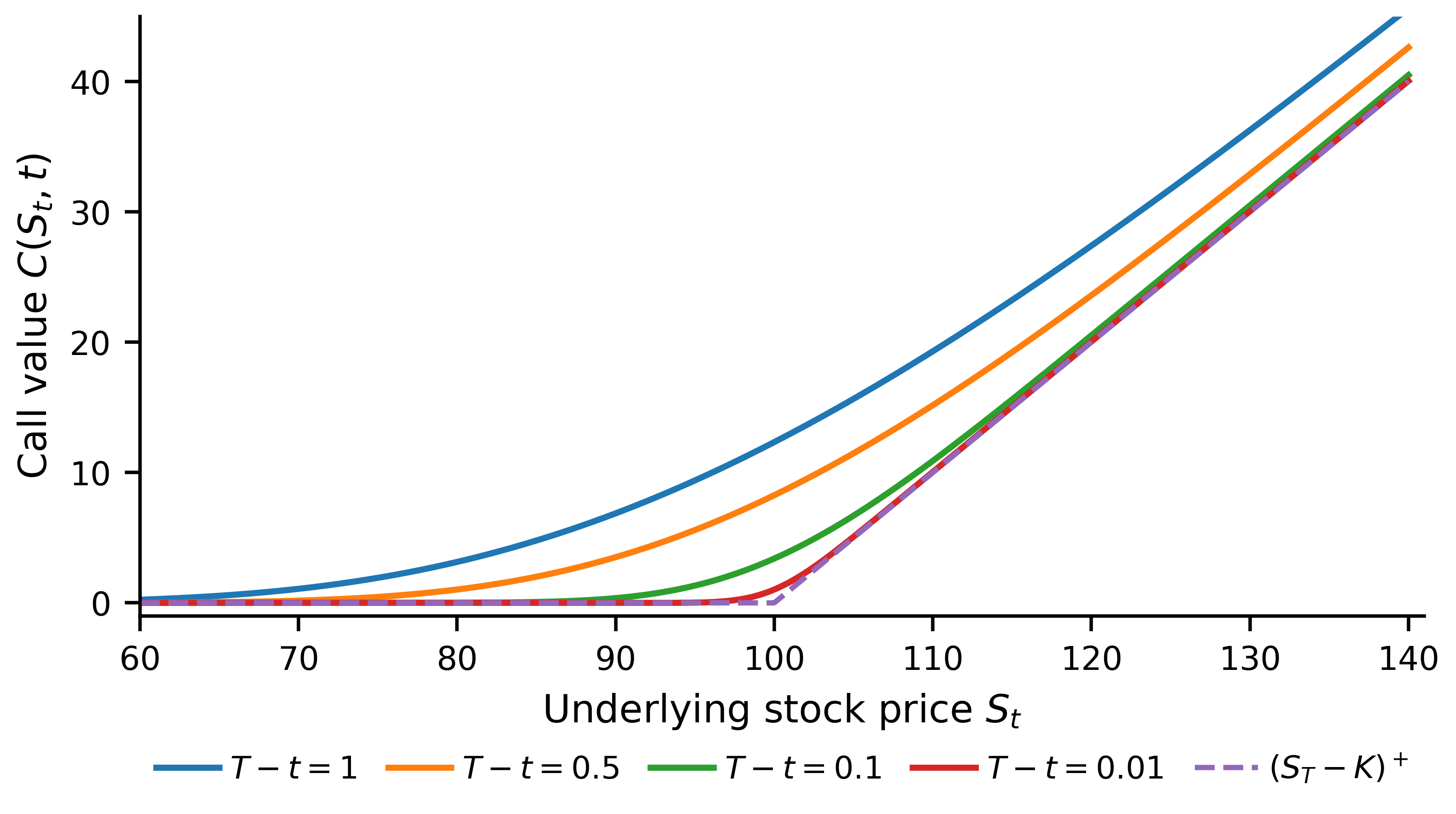
The standardized normal cumulative limits $d_1$ and $d_2$ also have useful interpretations. Differentiating the call formula with respect to $S$ — the extra terms from differentiating $N(d_1)$ and $N(d_2)$ cancel exactly — gives $C_S = N(d_1)$, so $N(d_1)$ is the option's delta and therefore the hedge ratio $\Delta_t = V_S$ in the replicating portfolio [3]. Under the risk-neutral measure, $N(d_2)$ is the risk-neutral probability that the call expires in the money, $P^*(S_T>K)$ [5]. As the time to maturity approaches zero, the option price curves converge to the sharp, non-differentiable boundary $(S_t-K)^+$ as shown in Figure 1.

Assumptions, Limitations, and the Risk-Neutral Interpretation§

Assumptions of the Model§

The derivation depends on several idealized assumptions about the market and the stock-price process. Each assumption enters the argument in a specific way:

1. Frictionless Markets: There are no transaction costs, borrowing/lending constraints, or differential taxes. Short-selling is permitted without restriction, and trading is continuous. Role: Permits continuous rebalancing and exact replication without transaction costs interfering with the hedge [1].
2. Constant Volatility: The volatility parameter $\sigma$ remains constant over the lifespan of the option. Role: Permits reduction to the standard constant-coefficient heat equation used for the closed-form solution.
3. Continuous Geometry: Under the GBM specification, the stock has continuous paths and quadratic variation $d[S]_t = \sigma^2 S_t^2 dt$. Role: Under the GBM specification, the quadratic variation has the stated form, allowing Itô's Lemma to be applied without jump terms.
4. Constant Risk-Free Rate: The risk-free borrowing and lending rate $r$ is constant over the life of the option. Role: Permits the continuous-compounding relation $d\Pi_t = r\Pi_t dt$ and produces the constant discount rate appearing in the PDE.
5. No Dividends: The underlying stock pays no dividends or distributions over the option's life. Role: Ensures that the self-financing relation $d\Pi_t = dV_t - \Delta_t dS_t$ does not require tracking discrete cash payouts from the stock or cash inflows into the portfolio.
6. Style of Option: The contract is a European-style option, meaning it can only be exercised at the final expiration date $T$. Role: Restricts the pricing problem to a fixed boundary at $T$, avoiding the free-boundary problem associated with early exercise.

Real-World Limitations§

In practice, the assumptions underpinning the Black--Scholes model are routinely violated, which directly impacts the accuracy of the formula:

• Volatility Smile and Skew (Violation of Constant Volatility): In real markets, implied volatility is not constant across strikes and maturities. Plotting implied volatility against the strike yields a u-shaped curve (the "volatility smile") or a downward slope (the "skew"). This observed smile and skew show that a single constant-volatility lognormal specification cannot reproduce observed option prices across strikes and maturities.
• Discrete Trading and Transaction Costs (Violation of Frictionless Markets): Perfect replication requires continuous rebalancing. In practice, bid-ask spreads and commissions make continuous rebalancing prohibitively expensive. Trading at discrete intervals introduces hedging errors, meaning the portfolio is never perfectly riskless over finite horizons.
• Path Discontinuities and Jumps (Violation of Continuous Asset Paths): Asset prices exhibit sudden, discontinuous jumps (e.g., during earnings announcements or market shocks). These jumps introduce discontinuous risk that cannot generally be eliminated by the continuous delta hedge used here.
• Dividend Distributions (Violation of No Dividends): Many stocks distribute dividends during the option's lifespan. Failing to account for these payouts leads to an overvaluation of call options, requiring a dividend-adjusted pricing equation [2].
• Term Structure of Interest Rates (Violation of Constant Risk-Free Rate): Interest rates vary over time. For long-dated options, a constant interest rate assumption fails to capture the interest rate risk of the discounting term, and time-varying interest rates may motivate time-dependent or stochastic interest-rate models.
• Early Exercise (Violation of European Style): Under the standard assumptions, the European formulation excludes early exercise, whereas American-style options lead to a free-boundary/optimal-stopping problem in which the exercise boundary must be determined. Under the standard assumptions, early exercise of an American call on a non-dividend-paying stock is suboptimal, so its value equals the corresponding European call value. For dividend-paying stocks, early exercise can become optimal.

Bridge to Martingale Pricing: The Risk-Neutral Measure§

While the replication argument developed in this note relies on dynamic hedging within the physical probability space, the pricing function $V(S, t)$ has an alternative probabilistic representation. By transitioning from the physical probability measure to an equivalent martingale measure, the appropriately discounted stock price process is a martingale. Under this representation, the drift of the stock price process is replaced by the risk-free rate $r$, and the option price admits a discounted risk-neutral expectation representation [3]. This motivates the next technical note in this series, where we will formalize equivalent martingale measures, Girsanov's Theorem, and the martingale representation theorem.

References§

1. Black, Fischer, and Myron Scholes. "The Pricing of Options and Corporate Liabilities." Journal of Political Economy 81, no. 3 (1973): 637–654.
2. Merton, Robert C. "Theory of Rational Option Pricing." Bell Journal of Economics and Management Science 4, no. 1 (1973): 141–183.
3. Shreve, Steven E. Stochastic Calculus for Finance II: Continuous-Time Models. Springer, 2004.
4. Karatzas, Ioannis, and Steven Shreve. Brownian Motion and Stochastic Calculus. Vol. 113. Springer, 1991.
5. Joshi, Mark S. The Concepts and Practice of Mathematical Finance. 2nd ed. Cambridge University Press, 2008.